Mikhail Naganov

Automatic Estimation of Signal Round Trip Delay, Part 2

In this post I explain how jack_delay estimator works. This utility is part of Linux JACK audio framework, its source code is available here.

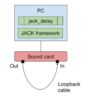
The utility is designed to measure round trip delay of sound cards, it calculates the delay from the phase of the returned signal. The output and the input of the sound card need to be connected by means of a loopback cable:

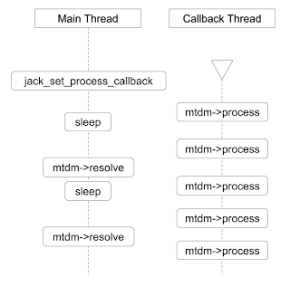
This is how the estimator is hooked up in the program. Jack offers a processing callback which is called on a high priority (Linux “real time”) dedicated thread, for low latency operation. This callback is registered by means of jack_set_process_callback API call. In the callback the delay estimator prepares and sends to output next audio buffer, and also receives a buffer of input data captured by the sound card. On the main thread the utility periodically checks and prints the current state of the delay estimator (mtdm):

What immediately occurred as strange to me is that the delay estimator class completely ignores the fact that it is being used in a multi-threaded setup—there are two threads that simultaneously read and write some of its fields, yet the latter are declared as ordinary variables. This gives the compiler a lot of freedom in rearranging the order of operations, which can affect correctness of the results. A correct modern solution would be to use atomic variables instead (but not a mutex, because the audio callback must call any function that could cause the thread to block, e.g. a function that attempts to acquire a mutex lock). Nevertheless, let’s ignore this shortcoming of the implementation and proceed to the delay estimation algorithm.

The delay estimator uses 13 sine signals. The actual frequencies of those signals depend on the sampling rate. The algorithm uses an expression 2 * π * k * f / 65536 for calculating the phase in radians for each sample of the sine waves it generates. For the main sine wave f equals to 4096 which emits the expression 2 * π * k * 1 / 16—that is, a period of 16 samples. Thus, for the sampling rate of 48 kHz, the main sine has frequency of 48 / 16 = 3 kHz.

In order to measure the phase of the sine wave that has returned back, the algorithm uses Discrete Fourier Transform formula expressed via Euler’s formula in terms of sine and cosine functions:

X(k) = Σ _{[n = 0..N - 1]} x(n) * (cos(2π * k * n / N) - j * sin(2π * k * n / N))

The algorithm only needs the main harmonic of the signal, so it sets k to 1. The algorithm also swaps “cos” and “sin” terms, and thus uses sines instead of cosines as the eigenvectors. This is done for convenience, as using cosines would require shifting the calculated phase by π / 2 because the source signal is a sine wave. This is the corresponding part of the source code:

c =  cosf (a);
s = -sinf (a);
F->xa += s * vip;
F->ya += c * vip;

After obtaining real and imaginary parts of the frequency domain complex function value, the algorithm uses a simple low-pass filter two times in order to smooth out any abrupt changes in the signal’s frequency domain form. Note—low pass filtering is not performed in the time domain, but rather in the frequency domain, thus the spectral composition of the signal remains the same.

The classical formula for a discrete time smoothing filter is:

y[i] = y[i - 1] + α * (x[i] - y[i - 1])

Below is the code where it is applied 2 times to real and imaginary parts:

F->x1 += _wlp * (F->xa - F->x1 + 1e-20);
F->y1 += _wlp * (F->ya - F->y1 + 1e-20);
F->x2 += _wlp * (F->x1 - F->x2 + 1e-20);
F->y2 += _wlp * (F->y1 - F->y2 + 1e-20);

The pair (x2, y2) is what ends up to be used to determine the phase of the sine wave. Note that the algorithm accumulates consecutive samples instead of building a smoothed vector. The smoothing parameter _wlp (same as α in the previous formula) is defined as 200 / sampling rate.

Since the algorithm doesn’t try to determine the phase at a certain point, but rather pretends that the analyzed sine is of an infinite duration, its resolution goes as high as 16 / 65536 part of a sample (65536 steps for the phase distributed over 16 samples of the main sine wave’s period). This is an extremely good resolution for all practical purposes!

But here we also have the multiplier ambiguity problem—since the sine function is periodic, the phase angle goes in circles, thus the maximum amount of phase shift that can be detected has the same time length as the period of the sine wave used. In other words, to detect a time delay of one second by using the phase of a single wave we would have to use a sine wave of 1 Hz frequency. Needless to say, it couldn’t be well reproduced anywhere but in a purely digital system. And even then, we would have to use large DFT windows in order to capture an entire period of the wave. This is by all means impractical.

The program uses a really clever approach—each of the additional 12 sine waves helps to determine the value of the corresponding bit of the delay value. Thus the range of the delay measurement gets extended to (2 ** 12) * 16 = 4096 * 16 = 65536 samples, which is more than a second when 48 kHz sampling rate is used.

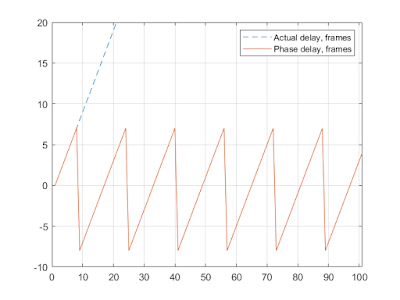
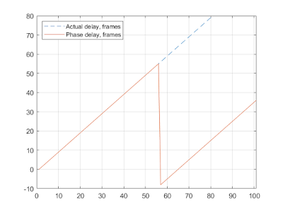
On the following graphs we can see how the phase rotation period doubles with each added sine wave. This is how the algorithm runs when it is using the first sine wave only:

As we can see, the phase of the sine wave follows the actual delay for the first 8 frames, then it resets to -8, grows back to 8, and so on. Now with the first two sine waves:

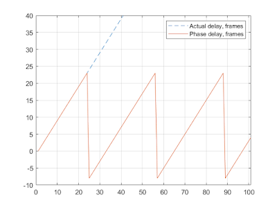
The period has increased twice—to 32, and the values go from -8 to 24. Now with the first 3 sine waves:

The period has increased twice once again, yielding the range of 64: from -8 to 56. And so on—when the algorithm uses all 13 sine waves the period becomes 65536 frames.

Let’s now take a closer look at what happens inside the analysis loop. For the first sine wave the delay calculation is straightforward:

d = atan2 (F->y2, F->x2) / (2 * M_PI);

Phase, which is in the range from -π to π, is normalized into the range [-0.5, 0.5]. For every other sine wave, the following formula is used:

p = atan2 (F->y2, F->x2) / (2 * M_PI) - d * F->f / f0;

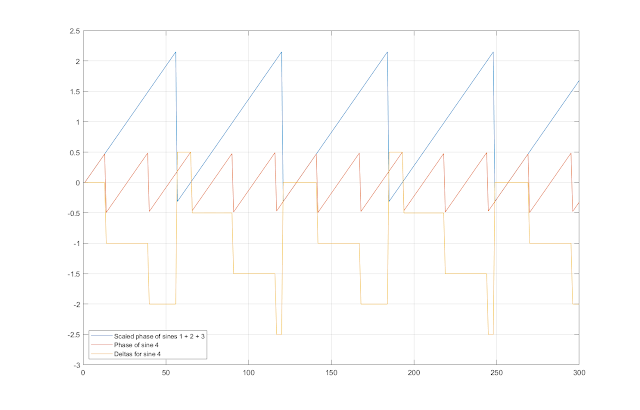
That’s the phase of the current sine wave, minus the value of the delay calculated so far, scaled by the the ratio of the current frequency to the frequency of the main sine wave (f0). For the 4th sine wave, the value of p changes as shown on the following figure:

Since the slopes of the phase functions match due to scaling, their difference is a step function. And because both phase functions are periodic, their difference is also periodic, with the period equal to the lowest common multiple of their periods. For example, the period of the combined wave formed by the sine waves 1, 2, and 3 is 64 samples. The period of the sine wave 4 (_freq[3].f) is 65536 / 2560 = 128 / 5 samples. Thus, the common period is 128 samples—that’s 2 * 64 = 5 * 128 / 5—this can be easily seen on the figure—both two periods of the blue graph and five periods of the red graph comprise one period of the yellow graph.

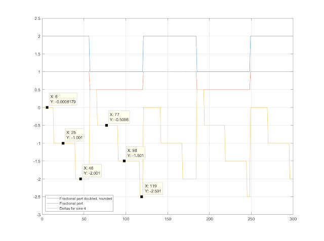
Another interesting property of the resulting yellow graph is that the values of the first half of its steps are close to whole numbers: 0, -1, -2, and another half is close to halves: 0.5, -0.5, -1.5, -2.5. By using this fact, the algorithm transforms the step function into a square wave:

Here is the corresponding code:

p -= floor (p);
p *= 2;
k = (int)(floor (p + 0.5));

First, the fractional part of the number is extracted. Note that because the values of the step function are not exactly whole numbers, and because they are negative, the resulting values may look surprising. For example, -0.0008179 gets “floored” to -1, and then, -0.0008179 - (-1) = 0.9992—as we can see, the red graph at X: 6 is almost 1. Anyways, the fractional part is a square wave with values very close to 0.5 or 1. The next two operations is doubling and rounding. The result is exactly 1 or 2—this is the blue graph. Note that depending on the input values, the fractional part can also have values close to 0 or 0.5, and the resulting square wave would be 0 or 1.

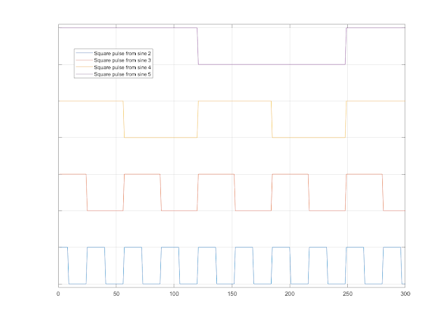
Below is the graph of the square wave functions calculated for the first four sine waves:

By carefully choosing the frequencies of the sine waves, the resulting square waves always double their frequency at the next step. Another important property of the sine waves is that they always start with 0 or 2 value. This way, the algorithm simply determines whether the value of the square wave is divisible by 2, and uses the result to add the next power of 2 to the value of the calculated delay:

m = 1;
...
d += m * (k & 1);
m *= 2;

Thus, the main “magic” of the algorithm is the choice of the frequencies for the supplemental sine waves. In fact, we have already seen the required ratio:

2 * 2 ** (i + 3) = M * (65536 / _freq[i].f)

For example, for i = 3 (sine wave 4) we have:

2 * 2 ** 6 = 2 * 64 = 5 * (65536 / 2560) = 5 * (128 / 5)

M in this case is 5. The algorithm also works if M is 3 (thus having _freq[3].f = 1536). Below is a complete list of the ratios for all the sine waves used (the divisors of 65536 are the values from the the _freq array in the program code):

* 2 ** 4 = 2 * 16 = 1 * 32 = 1 * (65536 / 2048)
* 2 ** 5 = 2 * 32 = 3 * 64 / 3 = 3 * (65536 / 3072)
* 2 ** 6 = 2 * 64 = 5 * 128 / 5 = 5 * (65536 / 2560)
* 2 ** 7 = 2 * 128 = 9 * 256 / 9 = 9 * (65536 / 2304)
* 2 ** 8 = 2 * 256 = 17 * 512 / 17 = 17 * (65536 / 2176)
* 2 ** 9 = 2 * 512 = 17 * 1024 / 17 = 17 * (65536 / 1088)
* 2 ** 10 = 2 * 1024 = 41 * 2048 / 41 = 41 * (65536 / 1312)
* 2 ** 11 = 2 * 2048 = 97 * 4096 / 97 = 97 * (65536 / 1552)
* 2 ** 12 = 2 * 4096 = 225 * 8192 / 225 = 225 * (65536 / 1800)
* 2 ** 13 = 2 * 8192 = 833 * 16384 / 833 = 833 * (65536 / 3332)
* 2 ** 14 = 2 * 16384 = 1793 * 32768 / 1793 = 1793 * (65536 / 3586)
* 2 ** 15 = 2 * 32768 = 3841 * 65536 / 3841

The choice of the ‘M’ coefficient is more or less arbitrary. It needs to be non-divisible by 2, obviously. Also, the choice of M affects the frequency of the sine wave, thus M must be chosen so that the frequency stays in the required range, and is unique.

The remaining code in the app deals with possible phase reversal in the audio system and with noise. I will explore the robustness of the algorithm in the following post.