Mikhail Naganov
Automatic Gain Control
This post is based on the Chapter 11 of the awesome book “Human and Machine Hearing” by Richard Lyon. In this chapter Dr. Lyon goes deep into mathematical analysis of the properties of the Automatic Gain Control circuit. I took a more “practical” route instead, and did some experiments with a model I’ve built in MATLAB based on the theory from the book.
What Is Automatic Gain Control?
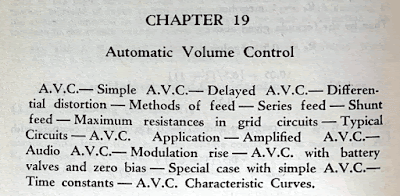
The family of Automatic Gain Control (AGC) circuits origins from radio receivers where it is needed to reduce the amplitude of the voltage received from the antenna in the case when the signal is too strong. In the old days the circuit used to be called “Automatic Volume Control” (A.V.C.), as we can see in the book on radio electronics design (“The Radiotron Designer’s Handbook”):
However, the earliest AGC circuits can be found in the human sensory system—they help to achieve the high dynamic range of our hearing and vision. In the hearing system the cochlea provides the AGC function.
The goal of AGC is to maintain a stable output signal level despite variations in the input signal level. The stability of the output is achieved by creating a feedback loop which “looks” at the level of the output signal, and makes necessary adjustments to the input gain of the signal at the entrance to the circuit. This is how this can be represented schematically:
Note that the “level” is a somewhat abstract property of the signal. What we need to understand is that “level” can be tied, based on our choice, either to the amplitude of the signal or to it’s power, and expressed either on a linear scale or on a logarithmic scale. There is also a somewhat arbitrary distinction between the “level” and the “fine temporal structure” of the signal. If we consider a speech signal, for example, it obviously has a high dynamic range due to fast attacks of consonant sounds. However, in AGC we don’t examine the signal at such a “microscopic” level. There is always a time constant which defines the speed of level variations that we want to preserve in the output signal.
We want the gain changes to be bound to the “slow” structure of the output signal, otherwise we will introduce distortions. The AGC Loop Filter is used to express the distinction between “fast” and “slow” by applying smoothing the measured level. The simplest way of smoothing is applying a low-pass filter (LPF). Although it’s common to define the LPF in terms of its cut-off frequency, another possible way is to use the “time constant”, which defines the former.
AGC vs. Other Systems
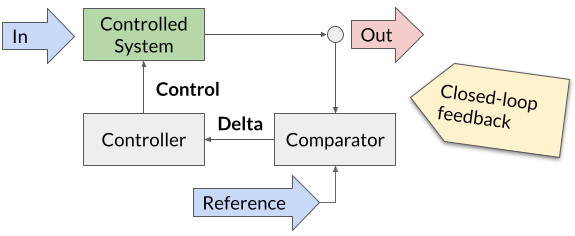
There are two classes of systems that are similar to AGC in their function. The first class is comprised of systems controlled by feedback—these systems are studied extensively by the engineering discipline called “Control Theory”. Schematically, a feedback-controlled system looks like this:
The big difference with AGC is that there is a “desired state” of the controlled system—this is what the control system is driving it towards. For example, in an HVAC system the reference is the temperature set by the user. In contrast, nobody sets the reference for an AGC circuit, instead, for any input signal that doesn’t change for some time, the AGC circuit settles down on some corresponding output level which is referred to as “equillibrium.”
Another class of systems that are similar to AGC are Dynamic Range Compressors, or just “Compressors”, frequently used when recording from a microphone or an instrument in order to achieve a more “energetic” or “punchy” sound. The main diffence of a compressor from an AGC is that compressors normally use the input signal for controlling their output—this approach is called “feed-forward”. Also, the design goal of the compressor is different from the design goal of an AGC, too—since it is used to “energize” the sound, adding harmonic distortions is welcome. Whereas, the design goal in AGC is to keep the level of distortions to minimum.
AGC Analysis Framework
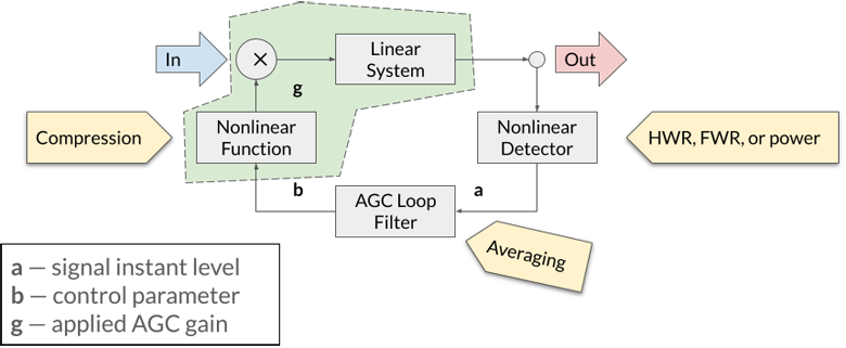
The schematic representation for the AGC we have shown initially isn’t very convenient for analysing it since the “controlled system” is completely a black box. Thus, the book proposes to split the controlled system into two parts: the non-linear part, which applies compression to the input signal, and the linear part which simply amplifies the compressed signal in order to bring it to the desired level. Note that since the compression factor is defined to be in the range [0..1], the compression always reduces the level of the input signal, sometimes considerably. Below is the scheme of the AGC circuit that we will use for analysis and modelling:
We label the outputs from the AGC blocks as follows:
- a is the measured signal level;
- b is filtered level;
- g is the compression factor.
In the book, Dr. Lyon uses the following function for calculating g from b:
g(b) = (1 - b / K)K, K≠0
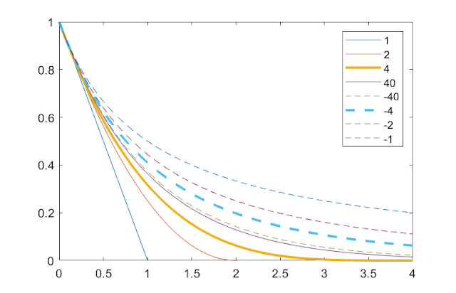
Below are graphs of this function for different values of K:
As the book says, the typical values used for K are +4 or -4.
AGC in Action
In order to provide a sense of the AGC circuit in action, I will show how the outputs from the blocks of the AGC change when it acts on an amplitude-modulated sinusoid. I used the same parameters for the input signal and the AGC circuit and obtained a result which looks very similar to the Figures 11.9 and 11.10 in the book.
The input signal is a sinusoid of 1250 Hz considered over a period of 1000 samples at the sampling rate of 20 kHz (that’s 50 µs). Below are the input an the output signals, shown on the same graph:
And this is how the outputs from the AGC loop blocks: a, b and c change:
The level analyzer is a half-wave rectifier, thus we only see positive samples of the output signal as the a variable. This output is being smoothed by an LPF filter with a cut-off frequency of about 16 Hz (10 ms—that’s the 1/5th of the modulation frequency), and the output is the b variable. Finally, the gain factor g is calculated using the compression curve with K = -4. The value of g never exceeds 1, thus to be able to see it on the graph together with a and b we have to “magnify” it. The book (and my model) uses the gain of 10 for the linear part of the AGC (this is designated as H) to bring the level of the output signal after compression on par with the level of the input signal.
My implementation of the AGC loop in MATLAB is rather straightforward. I decided to take an advantage of “function handles”, which are very similar to lambdas in other programming languages. The only tricky thing is to set the initial parameters of the AGC loop. Due to the use of feedback, there is a tricky situation with the values for the very first iteration, where the output isn’t available yet. What I’ve found after some experimentation is that we can start with zeroes for some of the loop variables and derive the values of other variables for them. Then we need to “prime” the AGC loop by running it on a constant level input. After a number of iterations, the loop enters the equillibrium state. This is how the loop looks like:
function out = AGC(in, H, detector, lpf, gain)
    global y_col a_col b_col g_col;
    out = zeros(length(in), 4);
    out(1, b_col) = 0;
    out(1, g_col) = gain(out(1, b_col));
    out(1, y_col) = H * out(1, g_col) * in(1);
    out(1, a_col) = detector(out(1, y_col));
    for t = 2:length(in)
        y = H * out(t - 1, g_col) * in(t);
        a = detector(y);
        b = lpf(out(t - 1, b_col), a);
        g = gain(b);
        out(t, y_col) = y;
        out(t, a_col) = a;
        out(t, b_col) = b;
        out(t, g_col) = g;
    end
end
And these are the functions for the half-wave rectifier detector and the LPF:
hwr = @(x) (x + abs(x)) / 2;

% alpha is the time constant of the LPF filter
lpf = @(y_n_1, x_n) y_n_1 + alpha * (x_n - y_n_1);
In order to be able to visualize the inner workings of the loop, the states of the intermediate variables are included into the output as columns.
Since the resulting gain is relatively high, reaching the value of
0.1 at the maximum, we use the compensating gain H=10. We can
also see that the gain factor g shows a dependency on the input
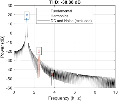
level. This leads to non-linearities of the output. Using MATLAB’s thd
function from the Signal Processing
Toolbox we actually
can measure it pretty easily on our sinusoid. Just as a reference, this
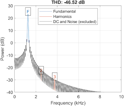
is what the thd function measures and plots for the input sinusoid
(only the 2nd and 3rd harmonics are shown):
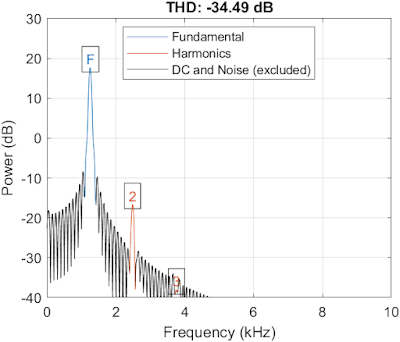
And this is what is shows for the output signal from our simulation:
As we can see, there is a non-negligible 2nd harmonic being added due to non-linearity of the AGC loop.
Experiments with the AGC Loop
What happens if we change the level detector from a half-wave rectifier
to a square law detector? In my model we simply need to replace the
detector function with the following:
sqr_law = @(x) x .* x;
Below are the resulting graphs:
What changes dramatically here is the level of compression. Since the square law “magnifies” differences between signal levels, high level signals receive a significant compression. As a result, I had to increase the compensation gain H on 5 orders of magnitude (that’s 40 dB).
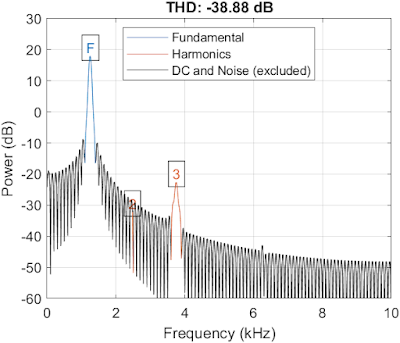
The behavior of the gain factor g still depends on the level of the input signal, so the circuit still exhibits a non-linear behavior. By looking at the THD graph we can see that in this case the THD is lower than of the half-rectifier AGC loop, and the dominating harmonic has changed to the 3rd:
Another modification we can try is change the time constant of the LPF filter. If we make the filter much slower, the behavior of the gain factor g becomes much more linear, however the output signal is even less stable than the input signal:
On the other hand, if we make the AGC loop much “faster” by shifting the LPF corner frequency upwards, it suppresses the changes in the input signal very well, but at cost of highly non-linear behavior of the gain factor g:
Can we achieve the higher linearity of the square law detector while still using the half-wave rectifier?
Multi-Stage AGC Loop
The solution dates back to the invention of Harold Wheeler who used vacuum tube gain stages for the radio antenna input. By using multiple stages, the compression can be increased gradually. Also, a stage with lower compression brings lower distortion. If we recall our formula for the compression gain (making K an explicit parameter this time):
g(b, K) = (1 - b / K)K, K≠0
We can see that by multiplying several functions that use smaller value of K we can achieve an equivalent of a single function with a bigger (in absolute value) K:
(g(b, -1))4 ~ g(b, -4)
Actually, if we change the definition of g to set the K as the divisor of b independently of the K power, we can obtain exactly the same function.
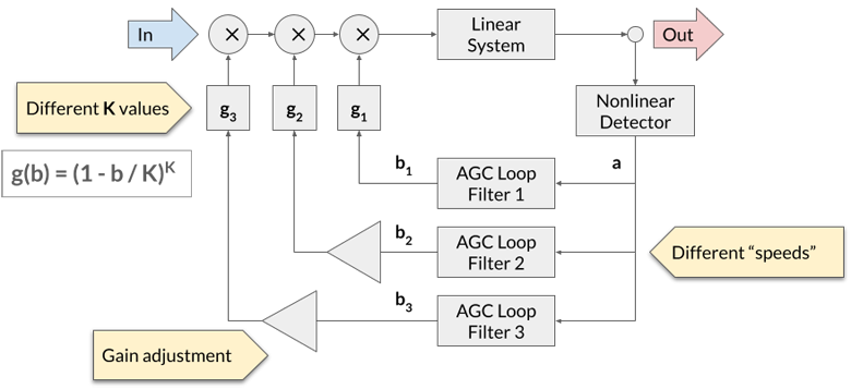
We can also vary the time constants of each corresponding LPF filter. This is how this approach looks schematically:
Each “slower” outer AGC loop reduces the dynamic range of the output signal, reducing the amount of the compression that needs to be applied for abrupt changes by inner “faster” loops, and thus keeping the distortion low.
I used 3 stages with the following LPF filters:
This is how the input / output and the loop variables look like:
We can still maintain a low compensating gain H in this case, and the behavior of the gain factor g is now more linear, and we can see this on the THD graph:
And here is the comparison of the outputs between the initial single stage approach with the square law and multi-stage approaches:
The multi-stage AGC yields a bit less compressed output, however it has less “spikes” on level changes.
Conclusions
It was interesting to explore the automatic gain control circuit. I’ve uploaded the MATLAB “Live” script here. I hope I can reimplement my MATLAB code in Faust to use as a filter for real-time audio. AGC is very useful for virtual conferences audio, as not all VC platforms offer gain control for participants, and when attending big conferences I often need to adjust volume.
